Missing outcomes imputation in bivariate meta-analysis

Padova EMPG Conference, 3 September 2025

Irene Alfarone, Filippo Gambarota, Massimiliano Pastore

Meta-analysis in psychology

A statistical technique to quantitatively summarize the results of multiple studies to derive a more precise effect estimate.
Various sources of heterogeneity: clinical, methodological, statistical

Multivariate meta-analysis

“[…] many clinical studies have more than one outcome variable; this is the norm rather than the exception. These variables are seldom independent and so each must carry some information about the others. If we can use this information, we should.” (Bland 2011)

Multivariate meta-analysis in psychology

Many psychological studies report multiple outcomes (Tyler, Normand, and Horton 2011)

MVMA allows for a joint estimation (Riley et al. 2017)
MVMA handles outcomes missing “by design” (Jackson et al. 2017)

Missing data

Rubin (1976) introduced a foundational framework distinguishing missing data mechanisms: Missing Completely At Random (MCAR), Missing At Random (MAR), Missing Not At Random (MNAR)

These mechanisms differ from missing data patterns, which refer to the observed structure of which values are present or absent.

Patterns = “What” is missing
Mechanisms = “Why” it is missing

Missing Completely At Random

MCAR: Missingness is unrelated to observed or unobserved data. The missing sample is a random subsample.

\[ P(M \mid Y, \phi) = P(M \mid \phi) \]

Missing At Random

MAR: Missingness depends on observed variables.

\[ P(M \mid Y, \phi) = P(M \mid Y_{obs}, \phi) \]

Missing Not At Random

MNAR: Missingness depends on unobserved variables (or both).

\[ P(M \mid Y, \phi) = P(M \mid Y_{mis}, \phi) \]

\[ P(M \mid Y, \phi) = P(M \mid Y_{obs}, Y_{mis}, \phi) \]

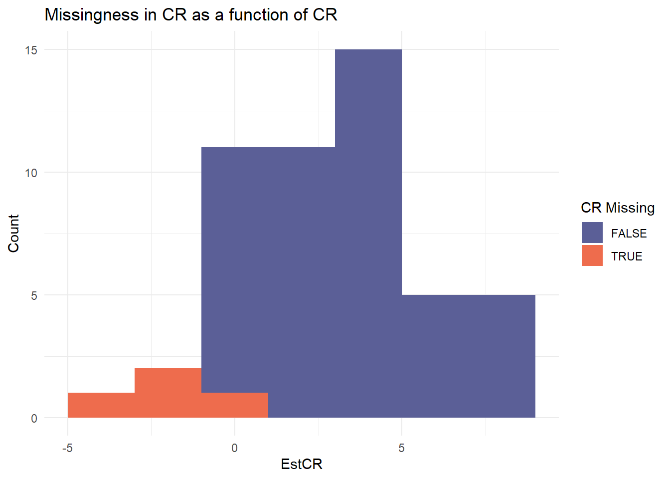
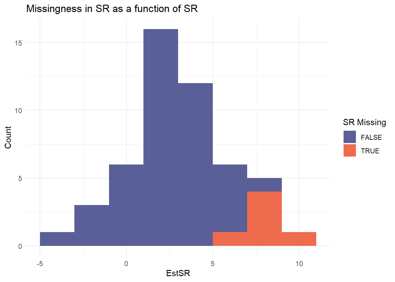
Multivariate meta-analysis and sensitivity analysis

What about MNAR outcome measures?
Pre-existing work on imputation of summary-level missing data (Lu 2023; Carpenter, Kenward, and White 2007; Viechtbauer 2022)
Delta-adjustment following multiple imputation of missing outcome (Fiero, Hsu, and Bell 2017)

Core Idea

Replace the unobserved outcomes with many plausible draws, then meta-analyse each imputed dataset and pool the results with Rubin’s rules.

Assume several donor distributions

e.g., Uniform, Normal, Multivariate Normal

Repeated stochastic single imputation

In each iteration
1. Draw missing effect estimates, SEs, and within-study cor
2. Fit a bivariate random-effects model (e.g., with mixmeta)
3. Store coefficients and vcov

Combine with Rubin’s rules
- Pool point estimates, between- & within-replicate variance
- Obtain bias, SE, CI coverage across replicates
Evaluation
- Bias and Coverage
- Sensitivity analysis for the estimates under different assumptions
- Easily interpretable plots with uncertainty intervals

Simulation study

50 studies, each with 100 participants
Two continuous outcomes:
- CR: Clinician Rating
- SR: Self-Report
Predictors: age, sex, treatment assignment
Random effects: bivariate normal with \(\rho = 0.7\)
Estimates obtained via Seemingly Unrelated Regression (SUR) (Zellner 1962; Riley, Tierney, and Stewart 2021)

MNAR mechanism

Missingness based on effect size estimates:
- CR: more likely missing when treatment effect is low
- SR: more likely missing when treatment effect is high
Conflict resolution: keep the one furthest from the mean

Imputation distributions

Missing outcomes were drawn from one of three distributions:

Normal with mean \(\in {−3, 0, 3}\)
Truncated multivariate normal (tmvn) with mean = (1, 5)
Uniform distribution from −100 to 100

Each condition was repeated 10,000 times, with:

Single stochastic imputation (×100)
Bivariate random-effects meta-analysis using mixmeta
Pooled estimates and variances via Rubin’s rule

Estimated CR with 95% CI

Estimated SR with 95% CI

Bias and Coverage for CR and SR

Bias and 95% CI Coverage for CR and SR by Imputation Distribution and Missingness
Imputation	Bias (CR)	Coverage (CR)	Bias (SR)	Coverage (SR)
normal (-3, -3)	-0.53	0.998	-1.12	0.492
normal (0, 0)	-0.12	1.000	-0.71	0.886
normal (3, 3)	0.27	1.000	-0.32	0.998
tmvn (1, 5)	-0.04	1.000	-0.01	1.000
uniform (0, 0)	-0.16	1.000	-0.75	1.000

Bias depends on missingness rule
Imputation from uniform distributions are conservative but imprecise
Imputation from truncate multivariate normal best performance, but relies on true model knowledge
In real data multiple assumptions should be tested

Application to real data

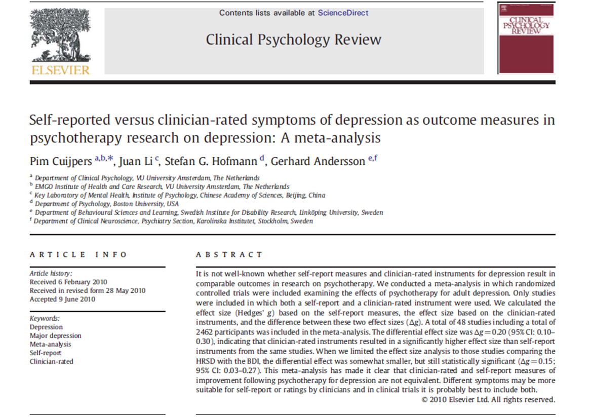
Cuijpers et al. (2010) collected data from 48 studies that measure depression on both a clinician rating (HRSD; Hamilton (1960)) and self-report scale (BDI; Beck et al. (1961)). The meta-analysis highlights a substantial difference between the patients’ and clinicians’ evaluations of depression, in favor of the clinician rating.

The dataset

37 studies from Appendix A (HRSD-17 and BDI outcomes, single control group, data from METAPSY database)
3 studies lacked post-treatment data
For multiple comparisons per study:
- Retained the highest mean difference
- BDI used to break ties

# A tibble: 6 × 7
  Study                                  N  EstCR  SECR EstSR  SESR Cor.ws
  <chr>                              <dbl>  <dbl> <dbl> <dbl> <dbl>  <dbl>
1 Arean et al. (1993)a                  49 -13.2   1.62  -5.5  1.89    0.7
2 Ayen and Hautzinger (2004)a           21  NA    NA    -14    1.75   NA  
3 Bowers et al. (1993)                  16  -3.1   1.52  -5.1  2.83    0.7
4 Bowman, Scogin, and Lyrene (1995)a    20  -7.1   3.17 -10.6  4.86    0.7
5 Brand and Clingempeel (1992)          53  -4.81  1.81  -2.6  2.58    0.7
6 Carpenter et al. (2008)               24   2.10  4.04  NA   NA      NA

Impute missing outcome measures using the package missmeta

Prepare distributions

I make explicit my assumptions regarding missing data, by exploring different scenarios.

library(missmeta)
library(tmvtnorm)
library(mvtnorm)

unif1 <- function(n) runif(n, min = -11, max = 11)
unif2 <- function(n) runif(n, min = -11, max = 11)

norm01 <- function(n) rnorm(n, mean = 0, sd = 6)
norm02 <- function(n) rnorm(n, mean = 0, sd = 6)

norm61 <- function(n) rnorm(n, mean = 6, sd = 6)
norm62 <- function(n) rnorm(n, mean = 6, sd = 6)

normn61 <- function(n) rnorm(n, mean = -6, sd = 6)
normn62 <- function(n) rnorm(n, mean = -6, sd = 6)

sigma <- matrix(c(6^2,
                 CorCov(6,6,0.7), 
                 CorCov(6,6,0.7), 
                 6^2), nrow = 2)

lower <- c(-100, -100)
upper <- c(100, 100)

mtv1 <- function(n) rtmvnorm(n, mean = c(-6, -6), sigma = sigma, lower = lower, upper = upper)[,1]
mtv2 <- function(n) rtmvnorm(n, mean = c(-6, -6), sigma = sigma, lower = lower, upper = upper)[,2]

Impute under different scenarios

Using the function genimp we generate 500 imputed values from each distribution.

imp1 <- list(unif1, norm01, norm61, normn61, mtv1)
imp2 <- list(unif2, norm02, norm62, normn62, mtv2)

out <- mapply(function(i1, i2) {
  genimp(
    df = dmnar,
    iter = 500,
    imp1 = i1,
    imp2 = i2,
    eff1 = "EstCR",
    eff2 = "EstSR",
    se1 = "SECR",
    se2 = "SESR",
    cor = "Cor.ws",
    N = "N",
    imprho = 0.6
  )
}, i1 = imp1, i2 = imp2, SIMPLIFY = FALSE)

Compute meta-analysis for each imputed dataset

Afterwards, we perform the chosen analyses on each imputed dataset. The user can autonomously choose the preferred meta-analysis package to conduct multivariate meta-analysis (e.g., metaSEM, mixmeta, metafor).

library(mixmeta)

outls = unlist(out, recursive = FALSE)

res = lapply(outls, function(data) {
  theta = cbind(data$EstCR, data$EstSR)
  Sigma = cbind(data$SECR^2, CorCov(data$SECR, data$SESR, data$Cor.ws), data$SESR^2)
  
  m = mixmeta(theta, S = Sigma, method = "ml")
  s = summary(m)
  ci = confint(m)
  
  results = data.frame(
  eff1 = s$coefficients[1,1],
  eff2 = s$coefficients[2,1],
  se1 = s$coefficients[1, 2],
  se2 = s$coefficients[2, 2],
  cov12 = s$vcov[1, 2],
  ci.lb1 = ci[1, 1], ci.ub1 = ci[1, 2],
  ci.lb2 = ci[2, 1], ci.ub2 = ci[2, 2]
  )
  
})

res <- do.call(rbind, res)

res <- split(res,  rep(1:5, each=500))

Summarize results for imputed datasets

With makepooldata we prepare the dataset to make it suitable for pooling estimates and standard errors obtained from the iterations using Rubin’s rules.

pooldata <- lapply(res, function(x) {
  makepooldata(data = x, effs = "eff", ses = "se", covs = "cov")
})

methods <- c("Uniform (-11, 11)", "Normal CR = 0, SR = 0", "Normal CR = 6, SR = 6",
               "Normal CR = -6, SR = -6", "Multivariate Normal (-6, -6)")

sumres <- mapply(function(p, label) {
  sumeth_multi(Q_mat = p$Q_mat, U_list = p$U_list, method = label)
}, p = pooldata, label = methods, SIMPLIFY = FALSE)

Plot the results

Conclusions

Via a simulation study and a real dataset we have shown the use of a flexible tool for imputing missing outcome data that:

Forces the researcher to make explicit the assumptions on the missing outcome data
Allows for imputation and robustness check of results under different scenarios
Can handle MNAR data
Is easy use and with missmeta quite forward to implement

Limitations

Results depend on the imputation distributions and parameters
Performance can drop if assumptions are far from reality (SR)
Slow at the moment if one has to test many assumptions

Future work

Increse computational efficiency
Extend to mor than two outcomes in multivariate meta-analysis
Explore proformance against existing imputation methods and sensitivity analysis techniques

References

Beck, A. T., C. H. Ward, M. Mendelson, J. Mock, and J. Erbaugh. 1961. “An inventory for measuring depression.” Archives of General Psychiatry 4 (June): 561–71. https://doi.org/10.1001/archpsyc.1961.01710120031004.

Bland, J. Martin. 2011. “Comments on ‘Multivariate Meta-Analysis: Potential and Promise’ by Jackson Et Al ., Statistics in Medicine: COMMENTARY.” Statistics in Medicine 30 (20): 2502–3. https://doi.org/10.1002/sim.4223.

Carpenter, James R., Michael G. Kenward, and Ian R. White. 2007. “Sensitivity analysis after multiple imputation under missing at random: a weighting approach.” Statistical methods in medical research 16 (3): 259–75. https://doi.org/10.1177/0962280206075303.

Cuijpers, Pim, Juan Li, Stefan G. Hofmann, and Gerhard Andersson. 2010. “Self-reported versus clinician-rated symptoms of depression as outcome measures in psychotherapy research on depression: a meta-analysis.” Clinical Psychology Review 30 (6): 768–78. https://doi.org/10.1016/j.cpr.2010.06.001.

Fiero, Mallorie H., Chiu-Hsieh Hsu, and Melanie L. Bell. 2017. “A Pattern-Mixture Model Approach for Handling Missing Continuous Outcome Data in Longitudinal Cluster Randomized Trials.” Statistics in Medicine 36 (26): 4094–4105. https://doi.org/10.1002/sim.7418.

Hamilton, Max. 1960. “A Rating Scale for Depression.” Journal of Neurology, Neurosurgery & Psychiatry 23: 56–61. https://doi.org/10.1136/jnnp.23.1.56.

Jackson, Dan, Ian R White, Malcolm Price, John Copas, and Richard D Riley. 2017. “Borrowing of Strength and Study Weights in Multivariate and Network Meta-Analysis.” Statistical Methods in Medical Research 26 (6): 2853–68. https://doi.org/10.1177/0962280215611702.

Lu, Min. 2023. “Computing Within-Study Covariances, Data Visualization, and Missing Data Solutions for Multivariate Meta-Analysis with Metavcov.” Frontiers in Psychology 14 (June). https://doi.org/10.3389/fpsyg.2023.1185012.

Riley, Richard D, Dan Jackson, Georgia Salanti, Danielle L Burke, Malcolm Price, Jamie Kirkham, and Ian R White. 2017. “Multivariate and Network Meta-Analysis of Multiple Outcomes and Multiple Treatments: Rationale, Concepts, and Examples.” BMJ, September, j3932. https://doi.org/10.1136/bmj.j3932.

Riley, Richard D, Jayne F Tierney, and Lesley A Stewart. 2021. Individual Participant Data Meta-Analysis. First Edition. Statistics in Practice. Wiley.

Rubin, Donald B. 1976. “Inference and Missing Data.” Biometrika 63 (3): 581–92. https://doi.org/10.2307/2335739.

Tyler, Kristin M., Sharon-Lise T. Normand, and Nicholas J. Horton. 2011. “The Use and Abuse of Multiple Outcomes in Randomized Controlled Depression Trials.” Contemporary Clinical Trials 32 (2): 299–304. https://doi.org/10.1016/j.cct.2010.12.007.

Viechtbauer, Wolfgang. 2022. “Multiple Imputation with the Mice and Metafor Packages [the Metafor Package].” https://www.metafor-project.org/doku.php/tips:multiple_imputation_with_mice_and_metafor.

Zellner, Arnold. 1962. “An Efficient Method of Estimating Seemingly Unrelated Regressions and Tests for Aggregation Bias.” Journal of the American Statistical Association 57 (298): 348–68. https://doi.org/10.1080/01621459.1962.10480664.