Missing outcomes imputation in bivariate meta-analysis

Psicostat Hands-On, 29 May 2025

Irene Alfarone, Filippo Gambarota, Massimiliano Pastore

Missing data: An overview

Rubin (1976) introduced a foundational framework distinguishing missing data mechanisms: Missing Completely At Random (MCAR), Missing At Random (MAR), Missing Not At Random (MNAR)

These mechanisms differ from missing data patterns, which refer to the observed structure of which values are present or absent.

Patterns = “What” is missing
Mechanisms = “Why” it is missing

MCAR

MCAR: Missingness is unrelated to observed or unobserved data. The missing sample is a random subsample.

\[ P(M \mid Y, \phi) = P(M \mid \phi) \]

MAR

MAR: Missingness depends on observed variables.

\[ P(M \mid Y, \phi) = P(M \mid Y_{obs}, \phi) \]

MNAR

Missingness depends on unobserved variables (or both).

\[ P(M \mid Y, \phi) = P(M \mid Y_{mis}, \phi) \]

\[ P(M \mid Y, \phi) = P(M \mid Y_{obs}, Y_{mis}, \phi) \]

Back to psychological meta-analysis

Meta-analyses in psychology often combine results reported on multiple instruments:

Correlated outcomes measuring same construct
Some outcomes often missing

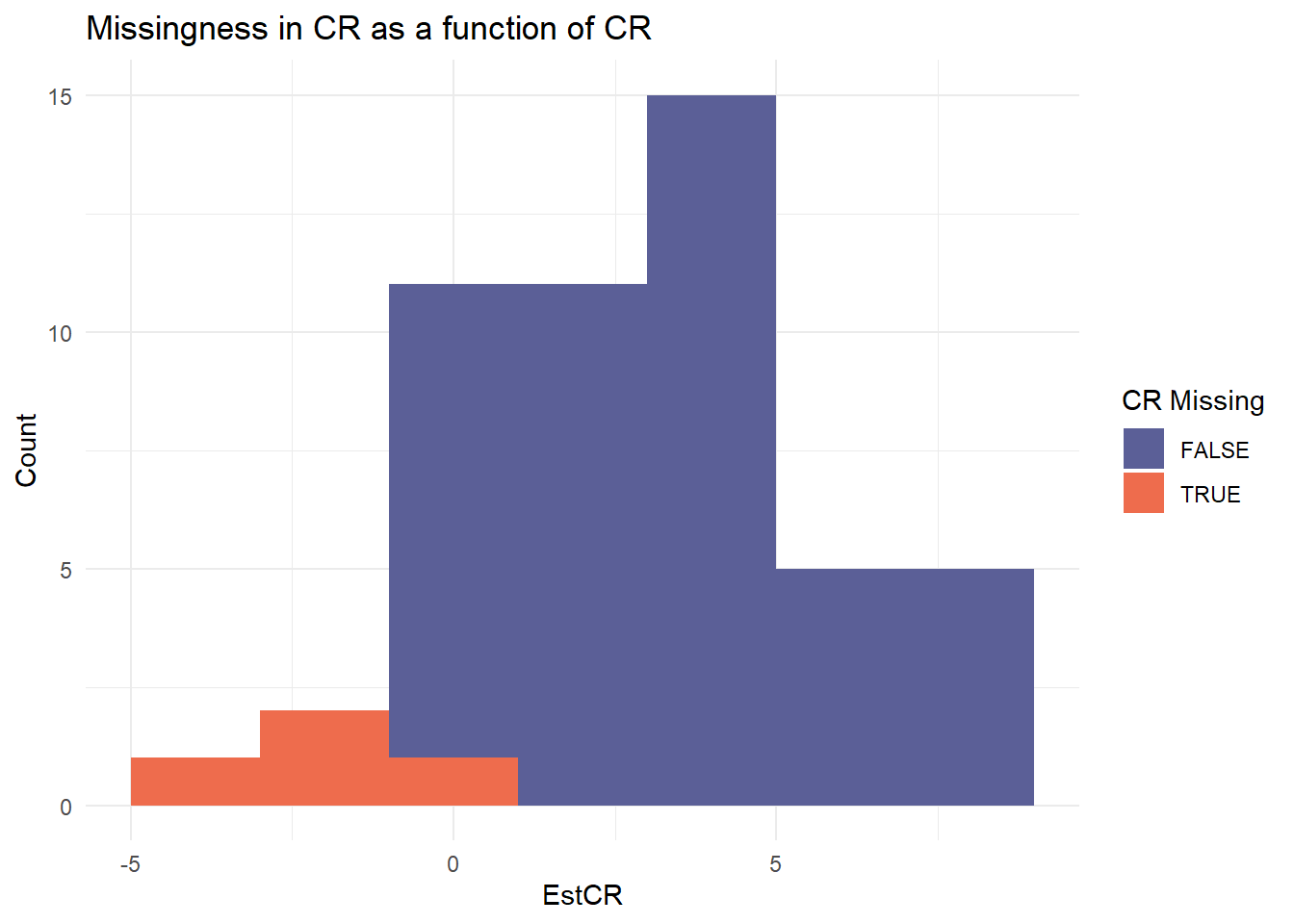
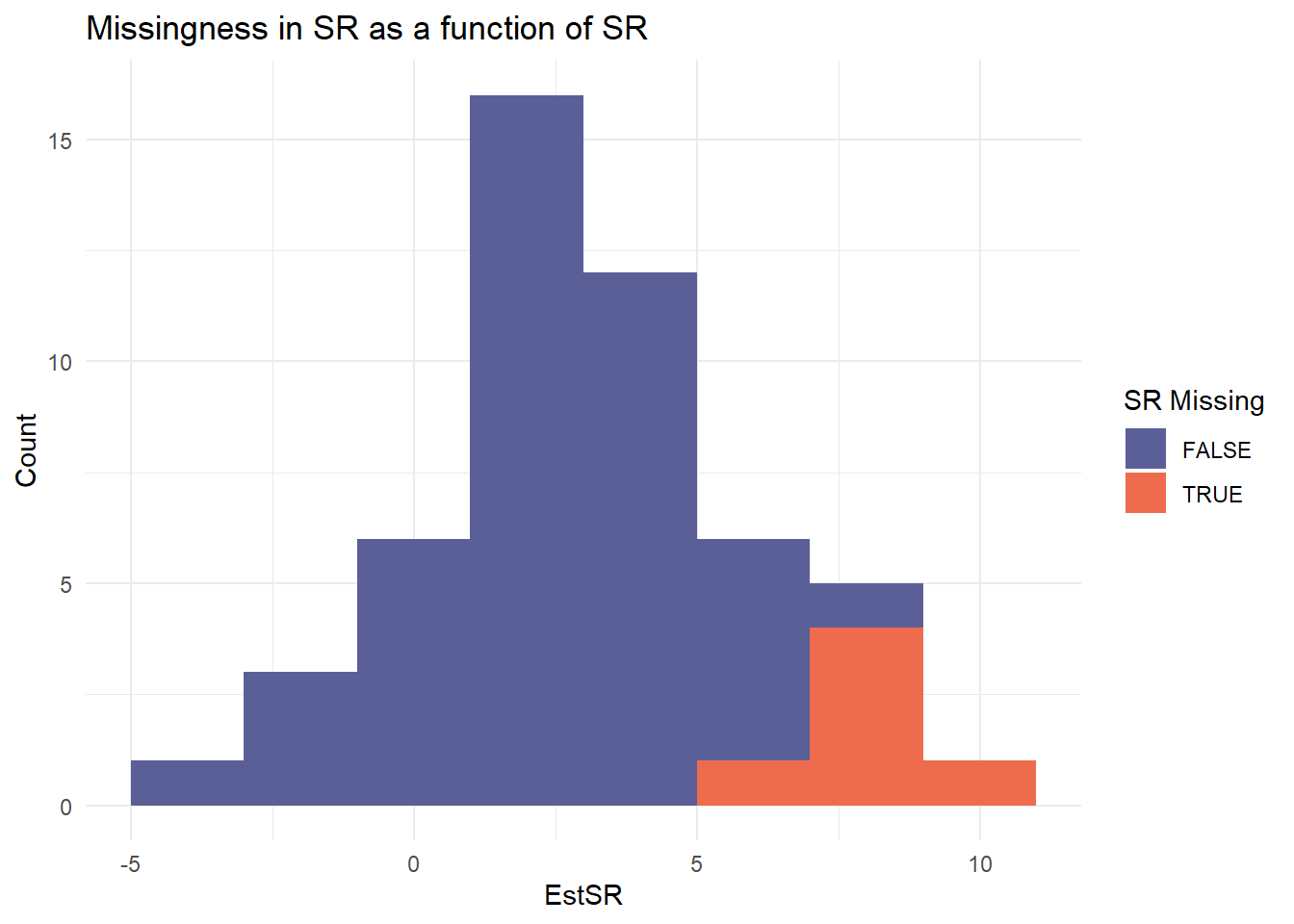
What if outcomes are missing not at random?

Core Idea

Replace the unobserved outcomes with many plausible draws, then meta-analyse each imputed dataset and pool the results with Rubin’s rules.

Assume several donor distributions

e.g., Uniform, Normal, Multivariate Normal (truncated)

Repeated stochastic single imputation

For every Monte-Carlo replicate
1. Draw missing effect estimates, SEs, and within-study cor
2. Fit a bivariate random-effects model (e.g., with mixmeta)
3. Store coefficients & vcov

Combine with Rubin’s rules
- Pool point estimates, between- & within-replicate variance
- Obtain bias, SE, CI coverage across replicates
Evaluation
- Bias and Coverage
- Sensitivity analysis for the estimates under different assumptions
- Easily interpretable plots with uncertainty intervals

Simulation study

50 studies × 100 subjects each
Outcomes:
- CR = Clinician Rating
- SR = Self Report
Estimates via Seemingly Unrelated Regression (SUR)

Missingness Mechanism (MNAR)

Logistic models on effect size estimates
Missingness depends on CR (positive bias) or SR (negative bias)

Imputation Strategy

We impute the datasets with random draws from pre-specified distributions imp1 and imp2, repeated iter = 100 times.

genimp = function(df, iter = 100,
                   imp1, imp2,
                   eff1 = "Eff1", eff2 = "Eff2",
                   se1 = "SE1", se2 = "SE2",
                   cor = "Cor.ws", N = "N",
                   imprho = 0.7) {
  results = vector("list", iter)
  
  for (i in seq_len(iter)) {
    dfi = df
    Nmiss1 = sum(is.na(dfi[[eff1]]))
    Nmiss2 = sum(is.na(dfi[[eff2]]))
    
    dfi[[eff1]][is.na(dfi[[eff1]])] = imp1(Nmiss1)
    dfi[[eff2]][is.na(dfi[[eff2]])] = imp2(Nmiss2)
    dfi[[cor]][is.na(dfi[[cor]])] = imprho
    
    comp = !is.na(dfi[[se1]]) & !is.na(dfi[[se2]])
    log_sig = cbind(
      log(dfi[[se1]][comp] * sqrt(dfi[[N]][comp])),
      log(dfi[[se2]][comp] * sqrt(dfi[[N]][comp]))
    )
    
    
    mu_hat    = colMeans(log_sig)
    Sigma_hat = var(log_sig)     
    
    miss = is.na(dfi[[se1]]) | is.na(dfi[[se2]])
    log_draw  = mvtnorm::rmvnorm(sum(miss), mean = mu_hat, sigma = Sigma_hat)
    sigma_imp = exp(log_draw)    
    
    idx_se1 = which(miss & is.na(dfi[[se1]]))
    idx_se2 = which(miss & is.na(dfi[[se2]]))
    
    dfi[[se1]][idx_se1] = sigma_imp[seq_along(idx_se1), 1] / sqrt(dfi[[N]][idx_se1])
    dfi[[se2]][idx_se2] = sigma_imp[seq_along(idx_se2), 2] / sqrt(dfi[[N]][idx_se2])
    
    results[[i]] <- dfi
  }
  
  results
}

Pooling with Rubin’s rules

After performing the chosen analysis on each imputed dataset, results from the bivariate meta-analysis are pooled using a procedure proposed by Rubin.

sum.meth = function(res, true1, true2) {
  m = nrow(res)
  Q_mat = cbind(res$eff1, res$eff2)
  Q_bar = colMeans(Q_mat)
  B = cov(Q_mat)
  
  U_list = lapply(1:m, function(i) {
    matrix(c(res$se1[i]^2, res$cov[i], res$cov[i], res$se2[i]^2), nrow = 2)
  })
  U_bar = Reduce("+", U_list) / m
  Tmat = U_bar + (1 + 1/m) * B
  se = sqrt(diag(Tmat))
  
  df = (m - 1) * (1 + diag(U_bar) / ((1 + 1/m) * diag(B)))^2
  
  ci1 = Q_bar[1] + c(-1, 1) * qt(0.975, df[1]) * se[1]
  ci2 = Q_bar[2] + c(-1, 1) * qt(0.975, df[2]) * se[2]
  
  data.frame(
    est_CR = Q_bar[1], est_SR = Q_bar[2],
    bias_CR = Q_bar[1] - true1,
    bias_SR = Q_bar[2] - true2,
    cover_CR = as.numeric(ci1[1] <= true1 && true1 <= ci1[2]),
    cover_SR = as.numeric(ci2[1] <= true2 && true2 <= ci2[2]),
    pci_lb_CR = ci1[1], pci_ub_CR = ci1[2],
    pci_lb_SR = ci2[1], pci_ub_SR = ci2[2]
  )
}

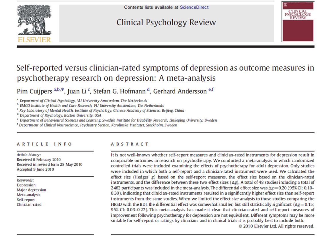
Cuijpers et al. (2010)

Cuijpers and colleagues collected data from 48 studies that measure depression on both a clinician rating (HRSD) and self-report scale (BDI).

The meta-analysis highlights a substantial difference between the patients’ and clinicians’ evaluations of depression, in favor of the clinician rating.

The dataset

We analyze a subset of studies that report either the HRSD (CR scale for depression) or the BDI (SR scale for depression).

Correlation between the HRSD and BDI is set at \(\rho = 0.7\) (yes, we could perform sensitivity analyses also for this…)

# A tibble: 6 × 7
  Study                                  N  EstCR  SECR EstSR  SESR Cor.ws
  <chr>                              <dbl>  <dbl> <dbl> <dbl> <dbl>  <dbl>
1 Arean et al. (1993)a                  49 -13.2   1.62  -5.5  1.89    0.7
2 Ayen and Hautzinger (2004)a           21  NA    NA    -14    1.75   NA  
3 Bowers et al. (1993)                  16  -3.1   1.52  -5.1  2.83    0.7
4 Bowman, Scogin, and Lyrene (1995)a    20  -7.1   3.17 -10.6  4.86    0.7
5 Brand and Clingempeel (1992)          53  -4.81  1.81  -2.6  2.58    0.7
6 Carpenter et al. (2008)               24   2.10  4.04  NA   NA      NA

Multivariate meta-analysis

Performed with mixmeta, comparable results also with metaSEM.

Call:  mixmeta(formula = theta, S = Sigma, method = "reml")

Multivariate random-effects meta-analysis
Dimension: 2
Estimation method: REML

Fixed-effects coefficients
    Estimate  Std. Error         z  Pr(>|z|)  95%ci.lb  95%ci.ub     
y1   -6.0612      0.5943  -10.1992    0.0000   -7.2259   -4.8964  ***
y2   -6.4748      0.8867   -7.3020    0.0000   -8.2127   -4.7369  ***
---
Signif. codes:  0 '***' 0.001 '**' 0.01 '*' 0.05 '.' 0.1 ' ' 1 

Random-effects (co)variance components
 Structure: General positive-definite
    Std. Dev    Corr
y1    2.8481      y1
y2    4.2588  0.6183

Multivariate Cochran Q-test for heterogeneity:
Q = 307.6164 (df = 61), p-value = 0.0000
I-square statistic = 80.2%

38 units, 2 outcomes, 63 observations, 2 fixed and 3 random-effects parameters
(3 units removed due to missingness)
   logLik        AIC        BIC  
-168.6260   347.2519   357.8063

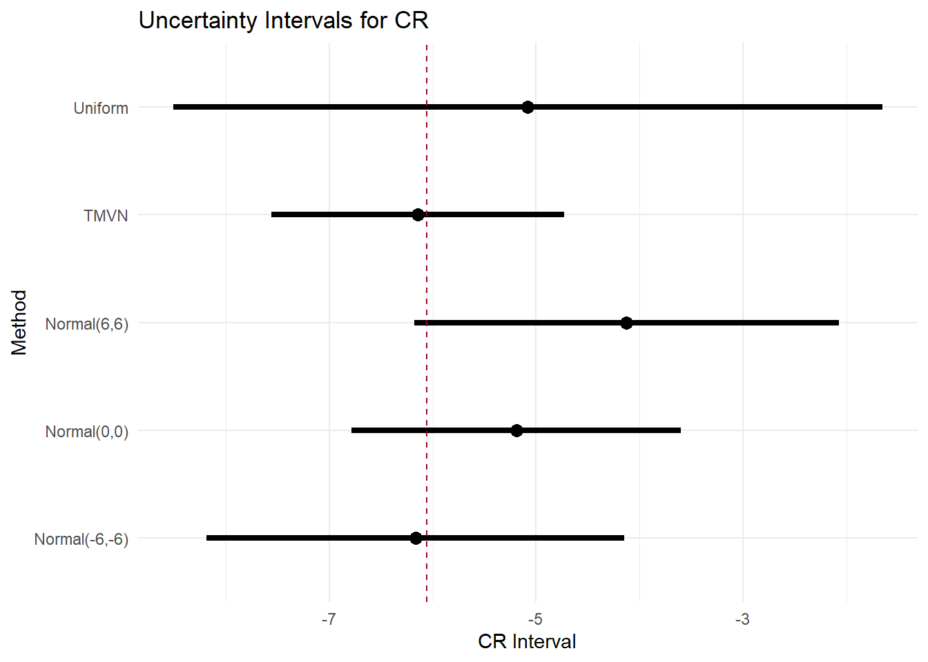
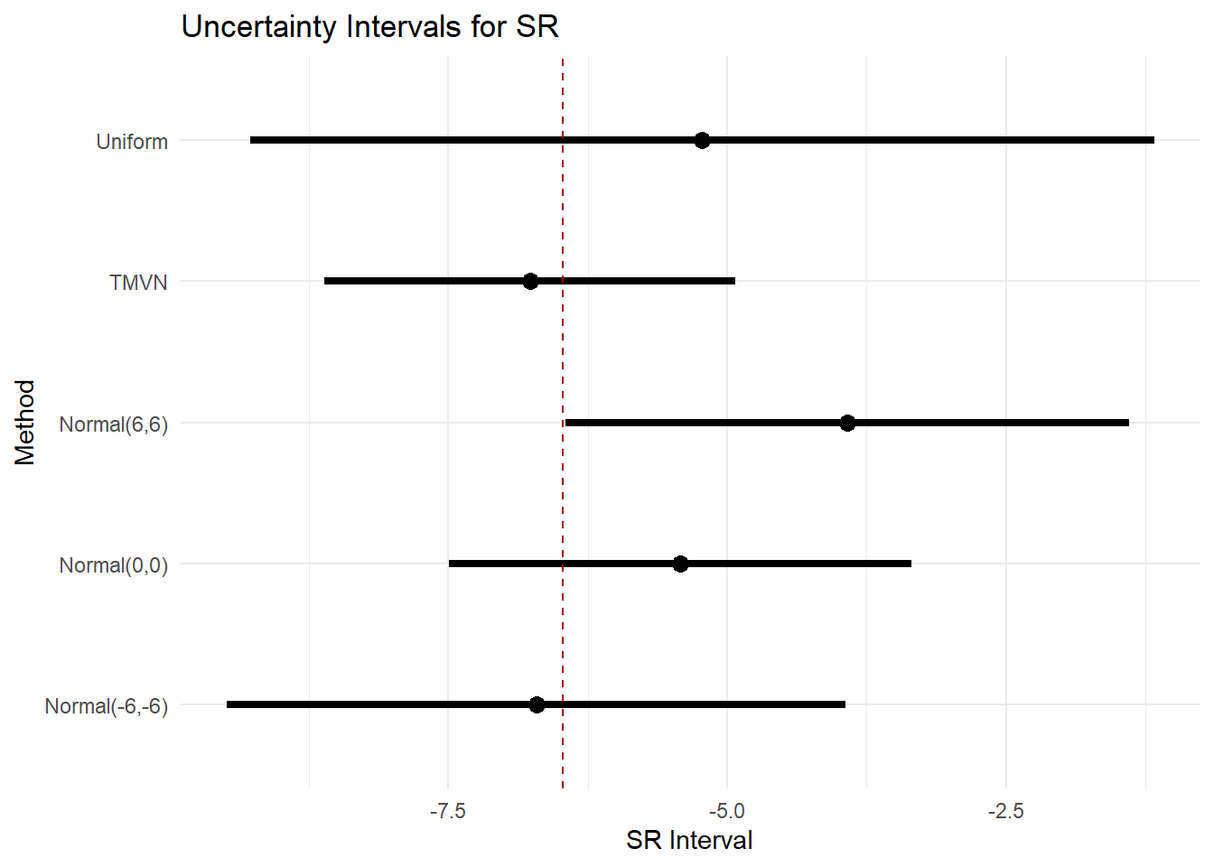
What if the outcomes are MNAR?

Then we imputed the missing HRSD and BDI outcomes with random draws from selected distribution (uniform, multivariate normal, normal) to reflect different assumptions on the missingness mechanisms.

The goal is to explore if the results are robust across assumptions (more or less conservative).

SPOILER!1!!1

It will be (soon) available an R package that allows the user to perform multivariate meta-analysis choices with different packages and choose her favourite distributions!