---
title: "Multiple testing in ANOVA and SEM"
author: "Enrico Toffalini, Irene Alfarone"
date: 'today'
format:
html:
code-fold: true
code-tools: true
editor: visual
---
## Overview
We present two simulated scenarios to illustrate the issue of multiple testing, by looking at false positive rates and power in:
- ANOVA
- Structural Equation Modeling (SEM)
## ANOVA
We simulated 5000 ANOVA with 3 binary predictors (A, B, C) and one continuous predictor (D), under H0 and H1 (y = 1 + 0.20\*C + residual).
```{r}
aovsim = function(niter = NA, h1 = NA, N = NA) {

  significanceCount = rep(NA,niter)
  ms = as.data.frame(matrix(NA, nrow = niter, ncol = 15))

  for(i in 1:niter){
    A = rbinom(N, 1, .5)
    B = rbinom(N, 1, .5)
    C = rbinom(N, 1, .5)
    D = rnorm(N, 0, 1)
    residual = rnorm(N, 0, 1)

    if(h1){
      y = 1 + 0.20*C + residual
    } else {
      y = 1 + residual
    }

    df = data.frame(A, B, C, D, y)

    ps = Anova(aov(y~A*B*C*D, data = df), type="II")$"Pr(>F)"
    ps = ps[!is.na(ps)]

    significanceCount[i] = sum(ps<0.05)
    ms[i, 1:length(ps)] = ps
  }

  colnames(ms) = rownames(Anova(aov(y~A*B*C*D,data = df)))[-nrow(Anova(aov(y~A*B*C*D,data = df)))]

  return(list(
    ms = ms,
    signCount = significanceCount,
    hist = hist(significanceCount),
    percSignCount = mean(significanceCount > 0)
  ))
}
```
```{r, message=FALSE}
library(car)

N = 1e+05
A = rbinom(N, 1, .5)
B = rbinom(N, 1, .5)
C = rbinom(N, 1, .5)
D = rnorm(N, 0, 1)
residual = rnorm(N, 0, 1)

y = 1 + 0.20*C + residual

df = data.frame(A, B, C, D, y)

Anova(aov(y~A*B*C*D, data = df), type="II")
```
```{r echo=F, eval=F, include=F}
mean(rowSums(nonull$ms[,colnames(nonull$ms)[!colnames(nonull$ms)%in%c("C")]]<0.05)>0)
correct = nonull$ms
for(i in 1:nrow(correct)) correct[i,] = p.adjust(correct[i,],method="fdr")
mean(rowSums(correct[,colnames(correct)[!colnames(correct)%in%c("C")]]<0.05)>0)
```
### Results of the simulation
| Metric | Value |
|----------------------------------------------------|-------|
| Power (before correction) | 88.8% |
| Power (after correction; FDR) | 60.6% |
| At least one false positive (before correction) | 49.7% |
| At least one false positive (after correction; FDR) | 6.8% |
: Under H1 (true effect of C)
## SEM
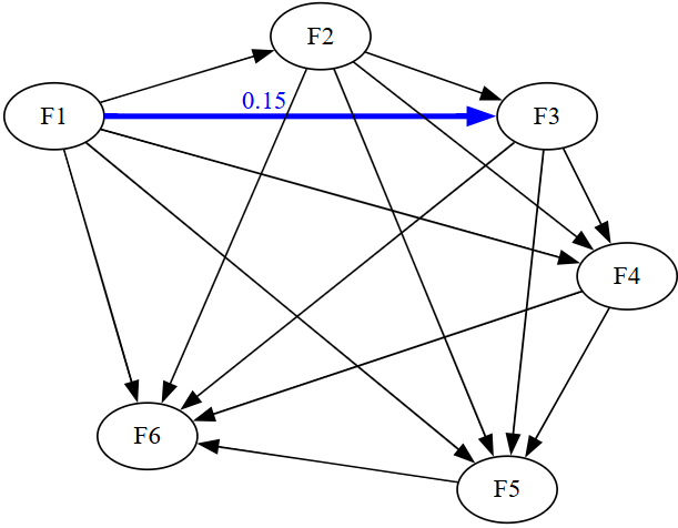
The simulated SEM model consists of six latent variables, each measured by ten indicators, with a true effect F3 \~ F1 under H1.
```{r, message = FALSE}
library(lavaan)
semsim = function(niter = NA, h1 = NA, N = NA, k = 6, w = 10, loading = 0.5) {

  generate_lavaan_model = function(k, w) {
    model_lines = sapply(1:k, function(f) {
      lhs = paste0("F", f, " =~ ")
      rhs = paste0("F", f, "_item", 1:w, collapse = " + ")
      paste0(lhs, rhs)
    })
    paste(model_lines, collapse = "\n")
  }

  significanceCount = rep(NA, niter)
  ms.sem = as.data.frame(matrix(NA, nrow = niter, ncol = 15))

  for(i in 1:niter){
    residual_sd = sqrt(1 - loading^2)
    latent_vars = matrix(rnorm(N * k), nrow = N, ncol = k)
    colnames(latent_vars) = paste0("F", 1:k)

    if (h1) {
      latent_vars[, "F3"] = 0 + 0.15*latent_vars[, "F1"] + rnorm(N, 0, 1)
    }

    observed_list = vector("list", k)
    for (j in 1:k) {
      indicators = matrix(
        loading * latent_vars[, j] + residual_sd * matrix(rnorm(N * w), nrow = N),
        nrow = N, ncol = w
      )
      colnames(indicators) = paste0("F", j, "_item", 1:w)
      observed_list[[j]] = indicators
    }

    df = as.data.frame(do.call(cbind, observed_list))

    modelM = generate_lavaan_model(k = 6,w = 10)
    model = paste(modelM,
                  "\n
              F6 ~ F1 + F2 + F3 + F4 + F5 \n
              F5 ~ F1 + F2 + F3 + F4 \n
              F4 ~ F1 + F2 + F3 \n
              F3 ~ F1 + F2 \n
              F2 ~ F1")

    fit = sem(model,df)
    pe = summary(fit)$pe
    ps = pe$pvalue[pe$op=="~"]

    significanceCount[i] = sum(ps < 0.05)
    #  print(paste("i:",i))
    #  print(paste("sign.count:",significanceCount[i]))
    ms.sem[i, 1:length(ps)] = ps
  }

  colnames(ms.sem) = paste(pe$lhs[pe$op == "~"], pe$op[pe$op == "~"], pe$rhs[pe$op == "~"])

  return(list(
    ms.sem = ms.sem,
    significanceCount = significanceCount,
    hist = hist(significanceCount),
    percSigPaths = mean(significanceCount > 0)
  ))
}
```
```{r echo=F, eval=F, include=F}
mean(rowSums(nonull.sem$ms.sem[,colnames(nonull.sem$ms.sem)[!colnames(nonull.sem$ms.sem)%in%c("F3 ~ F1")]]<0.05)>0)
correct = nonull.sem$ms.sem
for(i in 1:nrow(correct)) correct[i,] = p.adjust(correct[i,],method="fdr")
mean(rowSums(correct[,colnames(correct)[!colnames(correct)%in%c("F3 ~ F1")]]<0.05)>0)
```


### Results of the simulation
| Metric | Value |
|-----------------------------------------------------|-------|
| Power (before correction) | 94.6% |
| Power (after correction; FDR) | 72.8% |
| At least one false positive (before correction) | 49.6% |
| At least one false positive (after correction; FDR) | 6.1% |
: Under H1 (true path F3 \~ F1)


